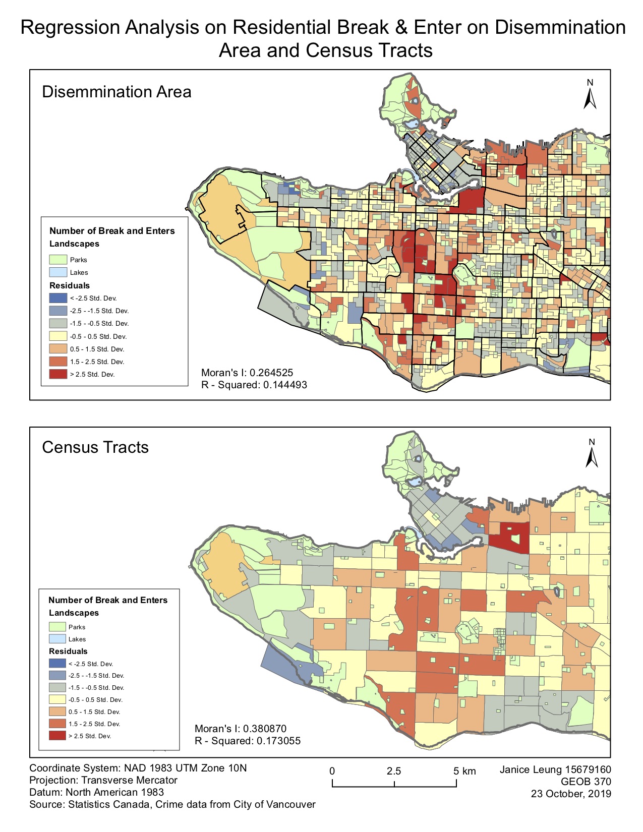
Ordinary Least Squares Regression Analysis
As seen from the maps above, there is a relatively more significant relationship between the values of the dependent variable (number of reported residential Break & Enter crimes) and the independent variable (median household income) in the DAs than the CTs. As demonstrated above, both the total private dwellings and the median household income in the DA are statistically significant. However, there is only the median household income in CT is statistically significant. This is due to the fact the DAs are divided into smaller areas, where less individual values are aggregated together, thus the relationship between the median household income and the total number of private households is a more statistically significant predictor of the break and enters in that area. However, for the CTs the area is larger and includes more individual values grouped together, thus only certain variables are significant in this regression equation as there are more variables that influence the predicted break and enters in each CT.
| Moran’s I | Significance Level (z score) | |
| Dissemination Areas (DA) | 0.264525 | 29.608577 |
| Census Tracts (CT) | 0.380870 | 9.265934 |
Spatial Autocorrelation
- The residuals are spatially autocorrelated, which means we do see a pattern of clustering, In terms of the distribution of residential B and E’s, the results suggests that the break and enter’s occurs in clusters. This means that if the neighbourhood has a significant difference to the expected number of break and enter’s, it is most likely that the area to the neighbourhood has around the same number of break and enter’s. In other words, if there is a high level of break and entering in one neighbourhood, it is most likely that there is also a high level of break and entering in the neighbourhoods nearby.
- Spatial autocorrelation does affect the result of the regression in terms of regression statistics, outside of the scale effect. However, spatial autocorrelation does not affect the regression parameters as the parameters are purely based on the values of the individual values in the data. When statistically significant spatial clustering residuals is present, it means that the regression model is missing some key variables explaining the relationship between the variables that we have chosen in our analysis. In our case, it means that there is more to take into consideration to predict the relative number of break and enters in each DA and CT other than just the median household income and also the total number of private household dwellings. This means that spatial autocorrelation “underperforms” the actual results of the regression and that there is more than just the median household income and also the total number of private household dwellings to define the values of residential break and enters.
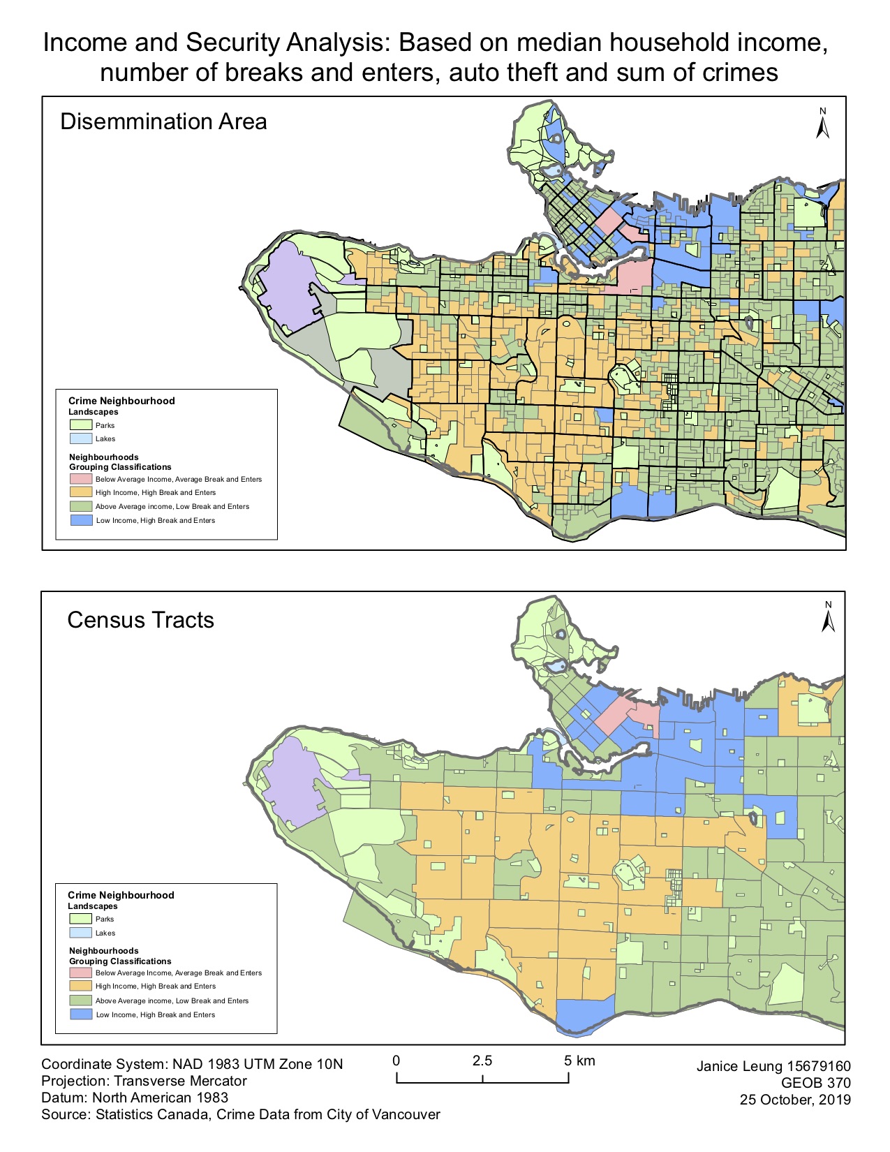
Grouping Analysis
- Both maps show the grouping of neighbourhoods into groupings to show which ones are the most problematic and which neighbourhoods we should mostly focus on. The different colors outlines the differences in income and if the number of residential break and enters in that area is higher or lower than expected. On the map, the yellow and green part generally refers to areas which are generally above the average income. The yellow refers to areas that have a high income and high break and enters while the green part is above average income and with low break and enters. The red and the blue part on the map refers to areas that generally have a lower income. The blue part on the map shows areas which have a low income and high break and enters while the red part is below average income and average break and enters.
- Based on both maps, we see areas of relative high income with high levels of break and enters are near to the centre of the map, at the middle of the city. However, there is a difference between the representation of data between CTs and DAs. We see variability present in areas such as downtown Vancouver where in the DAs the data shows that the area has low income and average break and enters. However in the CTs, the areas is seen as low income but high break and enters. This is most likely due to the modifiable areal unit problem (MAUP). The area in the CTs have a more diluted data, where areas with a high variability of data generally represent the whole area in CT and it is not what the area truly represents. It is better to have a DA map as a reference to determine the level of break and enters in each area in Vancouver.
Skills I Picked Up In This Assignment:
- Perform an OLS regression analysis on ArcGIS using open data catalogue from the City of Vancouver
- Explain and analyze spatial autocorrelation
- Manipulate and analyze census data
- Explain and show evidence of the ways in which MAUP impacts analyses
- Perform grouping analysis using ArcGIS
Learning Significance